

September 22nd, 2026
By Lotem Sella, CFA
You did it. Congratulations, you’ve retired and your golden years ahead of you. However, before you enjoy the fruits of your labor, you’ll have to make a couple of arrangements. First step, figure out the money problem. You know, the whole paying for bills now that paychecks have stopped coming problem. Second step, find ways to enjoy time in retirement. Now, I can’t help much with step two, unless you enjoy the occasional round of golf but step one, that is something your humble calculator-wielding author can assist with. So, let’s explore the Guyton-Klinger guardrails, a strategy designed to adjust retirement income as markets and portfolio values change.
To better understand the guardrail system, I invite you to take a trip to 1974 in my spreadsheet powered time machine. In the prior year, many important events occurred. Pink Floyd released Dark Side of the Moon, Richard Nixon told Americans he was not a crook, and the Arab oil embargo caused the price of oil to more than double a year later. These events were experienced by John and Jane Doe, a lovely couple, living in a lovely home, who just embarked on their retirement journey. Together, we will experience their financial highs and lows through the lens of a guardrail system designed to satisfy their income needs.
The Does have done an excellent job preparing for retirement and begin 1974 with an account worth $100k. This may not seem like a lot, but if we adjust the value for inflation, it would be worth $782.5k today. Sorry, did I mention there would be math?
Anyways, despite the worrying headlines, the Does feel confident in their retirement plan and are going to follow their financial advisor’s recommendation to implement the Guyton-Klinger guardrail system. At first, they considered following the 4% withdrawal rule, which stipulates their initial withdrawal amount would equal 4% of the account value and increased annually by inflation. However, their financial advisor has introduced the idea of a guardrail strategy and implementing a 5% initial withdrawal rate. This recommendation is based on a sophisticated Monte Carlo analysis, which suggests the Does can sustainably withdraw a higher amount.
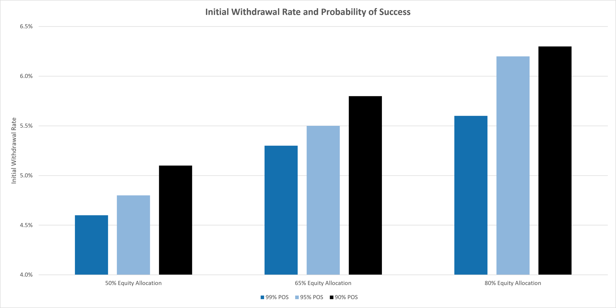
Source: Guyton-Klinger (2006)
The strategy will require the Does to follow a strict regimen of rules designed to minimize the likelihood of running out of money in retirement. When their portfolio experiences an upswing in value, they will receive a pay increase, but when the account falls in value, so will their monthly income.
Beyond the value of the portfolio, the Does decided to target an initial withdrawal rate of 5% while annually rebalancing their portfolio to allocate 65% to stocks, 25% bonds, and 10% in cash. The plan was dutifully executed by their amiable advisor and for the first decade produced the results shown below.

Source: Guyton-Klinger (2006), Shiller Data, Board of Governors of the Federal Reserve System
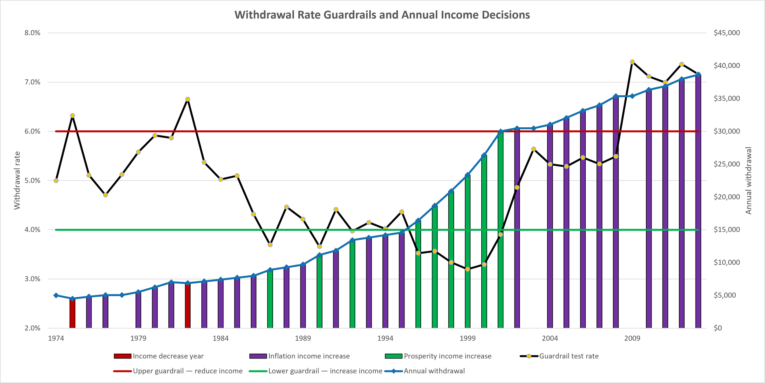
In hindsight, 1974 was an unfortunate year to begin retirement. The Arab oil embargo had a devastating effect on the rate of inflation, which grew at 12.3% that year. Additionally, the “Nifty Fifty” stock market bubble had already popped in the prior year, but the S&P 500 wasn’t finished with its decline. These events resulted in the withdrawal rate jumping from an initial 5% to 6.3%, as the same annual $5,000 withdrawal now represented a higher proportion of the account value. Per the Guyton-Klinger strategy, a 10% pay cut applied under the Capital Preservation rule of the guardrail system. Suffice to say, John and Jane were feeling uneasy at the start of retirement.
Despite the nerves, throughout the first decade the Does primarily experienced increases to their annual paycheck via the inflation adjustment of the strategy. However, in 1982 another capital preservation trigger occurred as the withdrawal rate had drifted to 6.7%. This time, the pay cut was only 2% as the rate of inflation was 8.9% in the prior year and counteracted the 10% haircut rule (see detailed explanation of rules below for more details).
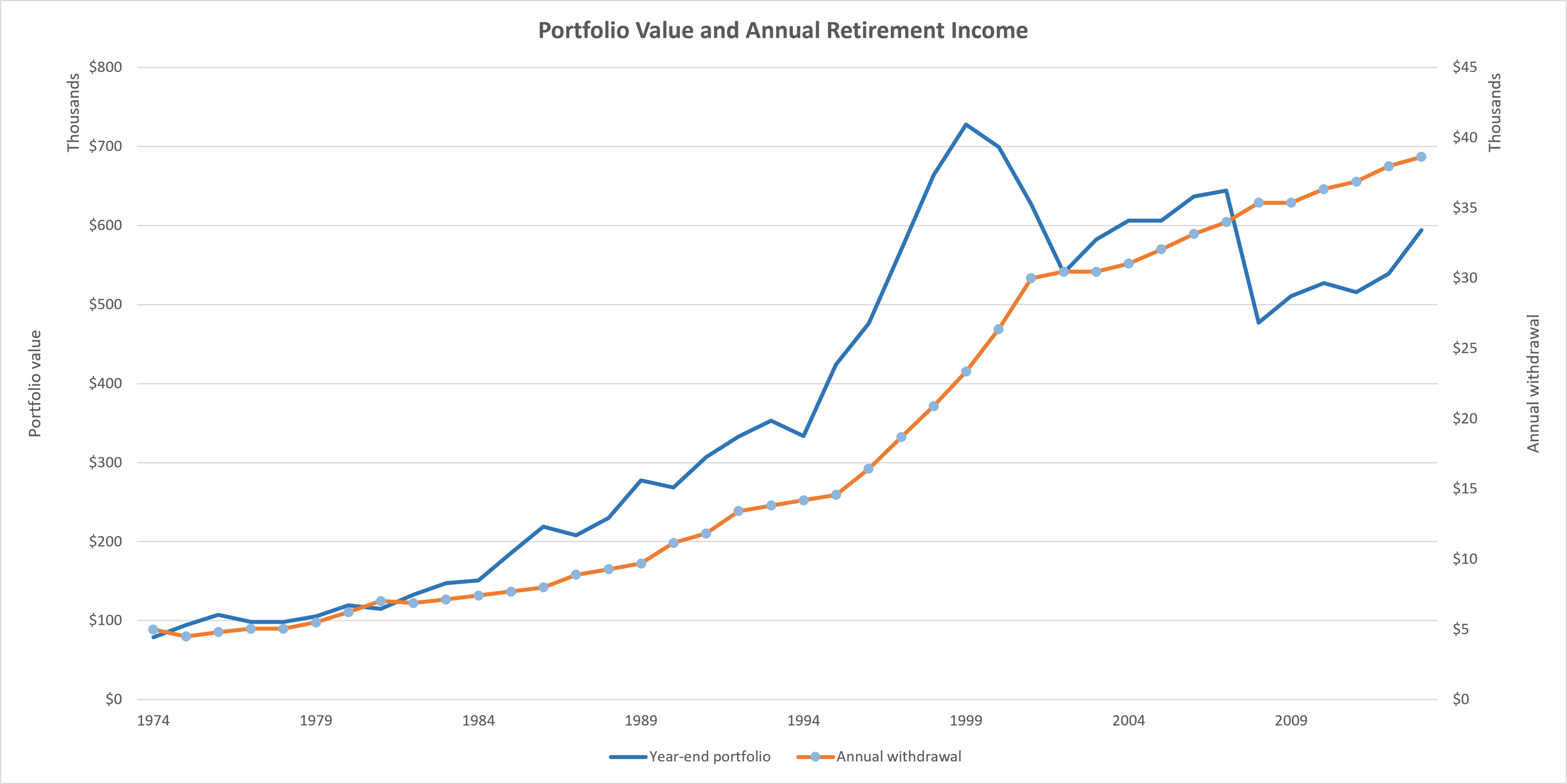
This was a tumultuous start for the Doe’s retirement. While they understood pay cuts occurred to preserve the portfolio, it was a difficult situation to stomach. Still, the family persevered and followed the strategy for 40 years.
Source: Guyton-Klinger (2006), Shiller Data, Board of Governors of the Federal Reserve System
By 2013, the Does had reached the conclusion of their spreadsheet simulated retirement. They witnessed the evolution of fashion in ways they never imagined, saw political leadership rotate in the White House, and best of all experienced the joy of watching their family grow. During this period, their portfolio expanded by over 400% even after taking out annual withdrawals. By the end they were grateful for the journey, despite it taking discipline to execute.
Source: Guyton-Klinger (2006), Shiller Data, Board of Governors of the Federal Reserve System
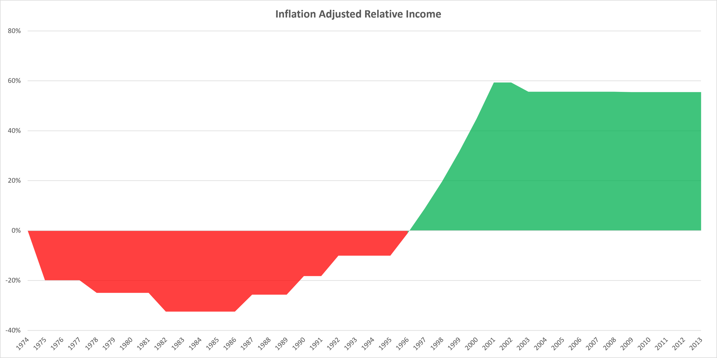
An especially difficult time to live through was the first two decades of retirement, when, on an inflation-adjusted basis, the Does had less spending power than when they started in 1974. During this period, the rate of inflation increased cumulatively by nearly 250% as the oil embargo of 1973 laid the groundwork for a chain reaction of price shocks. It wasn’t until 1982 when Paul Volker, the chairman of the Federal Reserve, “broke the back” of inflation by increasing interest rates and finally subdued the breakneck speed of price increases. By that point, the damage had already been done, and it would take another decade of strong asset returns to make the Does whole.
The Doe’s experience was chosen to highlight a worst-case scenario. Regardless of the withdrawal rule, most families choosing to retire in 1974 faced difficulties given the sequence of events of that era. Despite the difficulties, by the end of their retirement period the Does investment account never hit $0, and they were still able to take annual withdrawals. In many ways, the proof of a withdrawal system shouldn’t be in the average experience but rather in the worst-case scenario. Said differently, no one is going to be upset if they are wealthy when they turn 90, but being broke at that age presents difficult choices.
The Guyton-Klinger guardrail system isn’t perfect and with the advancement of financial modeling systems, investors can take advantage of different withdrawal techniques that may be more appropriate for their situation. What can be said is the Guyton-Klinger strategy progressed the state of distribution methods by introducing a rules-based decision hierarchy that dynamically adjusts investor’s annual income based on prevailing market conditions.
The Guyton-Klinger Rules:
Set an initial withdrawal rate expressed as a fraction of the account value. For example, an investor withdrawing $5k/year on a $100k portfolio has a withdrawal rate of 5%.
Withdrawals increase each year by the rate of inflation. However, there is no increase if two conditions are met:
Portfolio had a negative return in the prior year.
Withdrawal rate is greater than the initial withdrawal rate.
Capital perseveration rule; If the withdrawal rate is 20% greater than the initial withdrawal rate, reduce withdrawals by 10%.
This rule expires 15 years before the end of the retirement period
Prosperity rule: If the withdrawal rate is 20% less than the initial withdrawal rate, increase withdrawals by 10%.
Withdrawals are sourced from asset classes in the following order:
Equities, if overweight.
Fixed income, if overweight.
Cash
Fixed income
Equities
Source: Guyton-Klinger (2006), Shiller Data, Board of Governors of the Federal Reserve System
Methodology
This article presents a historical retirement illustration designed to show how the Guyton-Klinger decision rules would have affected a retiree beginning distributions in 1974.
The first table reports the annual mechanics for the first ten retirement years, including beginning portfolio value, the annual withdrawal, the change in income, the decision rule applied, total portfolio return, and inflation. The first chart extends the illustration across the full 40-year period and plots nominal portfolio value alongside annual withdrawals. The second chart expresses annual income relative to the initial withdrawal after adjusting for cumulative inflation. The final chart identifies the years in which income was reduced, increased only for inflation, or increased under the prosperity rule, and compares the current withdrawal rate with the 4% and 6% guardrails.
Scenario assumptions: The illustration uses the following starting conditions, timing conventions, and portfolio assumptions.
Retirement begins on January 1, 1974 and lasts 40 years, ending in 2013.
The hypothetical portfolio begins at $100,000 and the first annual withdrawal is $5,000, equal to a 5.0% initial withdrawal rate.
The target allocation is 65% equities, 25% bonds, and 10% cash. The portfolio is evaluated and rebalanced annually.
One full annual withdrawal is taken at the beginning of each retirement year, before that year’s investment returns are applied.
Historical monthly returns are compounded within each retirement year. The illustration is deterministic and uses the actual historical sequence beginning in 1974 rather than a Monte Carlo simulation.
The analysis is nominal unless a chart or table is explicitly labeled as inflation adjusted.
Withdrawal and portfolio decision rules
At each annual review, the current withdrawal rate is calculated by dividing the planned withdrawal by the beginning portfolio value. The following rules are then applied to determine the withdrawal and its source:
Inflation adjustment: the prior year’s withdrawal is increased by the prior year’s inflation rate unless the withdrawal rule or a guardrail adjustment applies. The illustration does not impose the 6% inflation cap used in the earlier 2004 framework, consistent with the 2006 Guyton-Klinger methodology.
Modified withdrawal rule: the inflation increase is skipped when the prior year’s total portfolio return was negative and the current withdrawal rate is above the initial 5.0% withdrawal rate. Missed inflation adjustments are not restored later.
Capital preservation rule: when the current withdrawal rate rises more than 20% above the initial rate, meaning above 6.0%, the annual withdrawal is reduced by 10%. This rule is discontinued for the final 15 years of the 40-year planning period.
Prosperity rule: when the current withdrawal rate falls more than 20% below the initial rate, meaning below 4.0%, the annual withdrawal is increased by 10%.
Withdrawal sourcing and rebalancing: cash needs are funded first from overweight equities, then overweight fixed income, followed by cash, remaining fixed income, and finally equities. The remaining portfolio is rebalanced to the 65%/25%/10% target allocation at the annual review.
Return and inflation data
Equity returns are derived from Robert Shiller’s historical U.S. stock-market data using prices and dividends. Bond returns are also derived from the Shiller dataset and are estimated using a constant-duration methodology. Cash returns use the 1-year Treasury interest-rate series from the Federal Reserve Bank of St. Louis and apply the same constant-duration methodology. Inflation is measured using the Consumer Price Index series contained in the Shiller historical dataset.
At a high level, a constant-duration methodology treats the bond and cash allocations as portfolios that maintain a consistent interest-rate sensitivity through time. As each period passes, the holdings are effectively rolled or rebalanced back to the target duration rather than allowing a single security to shorten naturally toward maturity. Estimated total returns therefore reflect both the income earned from the prevailing yield and the price effect of changes in interest rates, while maintaining a comparable maturity and duration profile across the historical period.
Monthly stock, bond, cash, and inflation observations are converted into total-return and inflation series and compounded within each calendar year. The weighted asset-class returns are then applied to the portfolio after the beginning-of-year withdrawal and the applicable Guyton-Klinger decision rules.
No taxes, advisory fees, fund expenses, transaction costs, bid-ask spreads, or investor behavior changes are modeled. Results therefore illustrate the mechanics of the specified historical scenario and should not be interpreted as a forecast or as a replication of every assumption used in the original Guyton and Guyton-Klinger research.
Disclosure
This article is provided for educational and informational purposes only and should not be construed as investment, tax, legal, or financial planning advice.
The examples are hypothetical and based on historical data. Past performance does not guarantee future results. Future market returns, inflation, interest rates, tax rules, investment costs, and investor behavior may differ materially from the historical periods discussed.
The retirement examples use simplified assumptions and do not reflect the circumstances of any particular investor. Actual retirement income planning should consider factors such as life expectancy, taxes, Social Security claiming decisions, spending flexibility, healthcare costs, required minimum distributions, portfolio expenses, and personal risk tolerance.
References to Jonathan Guyton and William Klinger’s research and the Guyton-Klinger guardrail framework are intended to summarize historical findings. They should not be interpreted as a recommendation that any specific withdrawal rate, asset allocation, or retirement income strategy is appropriate for every investor.
Sources
Guyton, Jonathan T. (2004). Decision Rules and Portfolio Management for Retirees: Is the “Safe” Initial Withdrawal Rate Too Safe?. Journal of Financial Planning. Available at: https://cornerstonewealthadvisors.com/wp-content/uploads/2014/09/2004-JFP-Article.pdf
Guyton, Jonathan T., and William J. Klinger (2006). Decision Rules and Maximum Initial Withdrawal Rates. Journal of Financial Planning. Available at: https://www.financialplanningassociation.org/sites/default/files/2021-11/2006%20-%20Guyton%20and%20Klinger%20-%20Decision%20Rules%20and%20SWR%20%281%29.PDF
Shiller, Robert J.. U.S. Stock Markets 1871–Present and CAPE Ratio Data. Yale University. Available at: https://shillerdata.com/
Board of Governors of the Federal Reserve System (US). Market Yield on U.S. Treasury Securities at 1-Year Constant Maturity, Quoted on an Investment Basis [GS1]. FRED, Federal Reserve Bank of St. Louis. Available at: https://fred.stlouisfed.org/series/GS1
Pfau, Wade D.. The Original Retirement Spending Decision Rules. Retirement Researcher. Available at: https://retirementresearcher.com/original-retirement-spending-decision-rules/
Fitzpatrick, Justin (2024). Why Guyton-Klinger Guardrails Are Too Risky for Most Retirees (And How Risk-Based Guardrails Can Help). Kitces.com. Available at: https://www.kitces.com/blog/guyton-klinger-guardrails-retirement-income-rules-risk-based/
